LAB 11
Localization (Simulator)

Lab 11 was the first localization lab, which is a focus of the last part of the course. In this lab, we implemented grid localization on a virtual robot in the simulator using the Bayes Filter, while the robot follows a preprogrammed trajectory in grid. This lab helped me learn a lot about using a simulator and about the Bayes filter, which I didn't have any experience with before. The codebase equipped with the simulator, mapper and other things, along with all the information provided in the lab handout and the skeleton Jupyter notebook was extremely helpful in completing this lab, as it reduced our task to simply understanding and implementing the Bayes filter.

Background

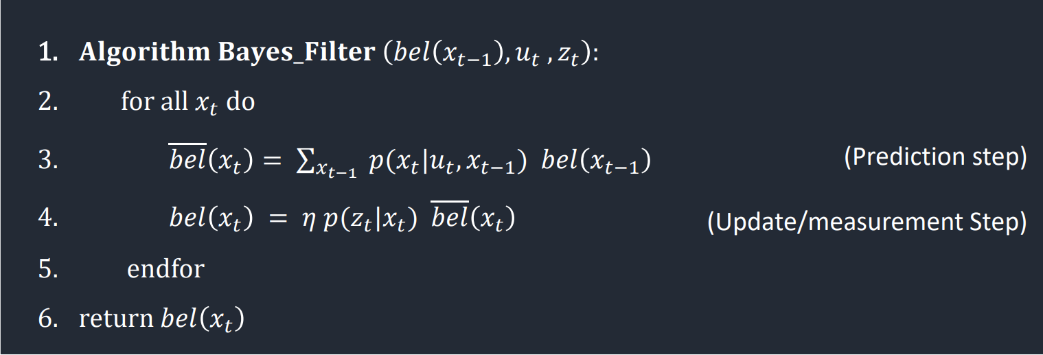
The Bayes Filter, as discussed in class, provides a probabilistic Robot-Environment model based on the belief distribution of the robot calculated with the help of measurements and control data. The filter can be broken down in two main steps, the prediction and the update, which are shown below with the Bayes filter algorithm. In the prediction step, the robot takes its prior belief about its location in the grid, and predicts is current location based on the movement that it went through (motion model). To update its belief, the robot takes a sensor measurement and compares that with the previously taken sensor measurement from every state in the grid to find the likelihood of it being in each state.

The robot state is 3-dimensional and defined by (x, y, angle) which have the following ranges in the state space.

- x: [-1.6764, +1.9812) meters or [-5.5, 6.5) feet
- y: [-1.6764, +1.9812) meters or [-5.5, 6.5) feet
- angle: [-180°, 180°]

In order to practically implement the Bayes filter, we need to discretize the robot state space into grid cells. For these labs, we do so for x and y with the help of 1ft tile markers in the room, and for angles, by splitting into 18 20°-increments, resulting in a discrete grid space of the size (12, 9, 18)

Prediction Step

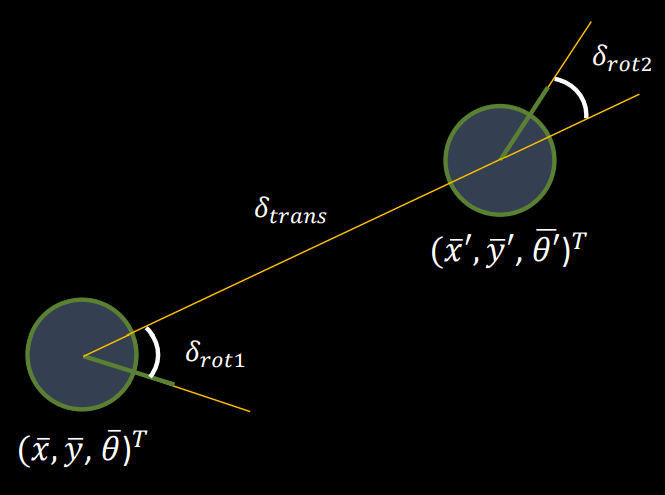
For the prediction step, we need to first define the robot motion model. In this lab and the next, the motion model of the robot is described as a Gaussian distribution centered at the motion measured using odometry of the robot. The motion control of the robot is described as a tuple of (rotation_1, translation, rotation_2) which was discussed in Lecture 18. We define a function compute_control() to find this motion control from the previous and current odometry poses.

def compute_control(cur_pose, prev_pose):
    """ Given the current and previous odometry poses, this function extracts
    the control information based on the odometry motion model.

    Args:
        cur_pose  ([Pose]): Current Pose
        prev_pose ([Pose]): Previous Pose 

    Returns:
        [delta_rot_1]: Rotation 1  (degrees)
        [delta_trans]: Translation (meters)
        [delta_rot_2]: Rotation 2  (degrees)
    """

    # Calculate the direction of cur_pose from prev_pose 
    dir_trans = degrees(atan2(cur_pose[1] - prev_pose[1], cur_pose[0] - prev_pose[0]))

    # First rotation
    delta_rot_1 = mapper.normalize_angle(dir_trans - prev_pose[2])

    # Translation distance 
    delta_trans = sqrt((cur_pose[1] - prev_pose[1])**2 + (cur_pose[0] - prev_pose[0])**2)

    # Second rotation
    delta_rot_2 = mapper.normalize_angle(cur_pose[2] - dir_trans)

    return delta_rot_1, delta_trans, delta_rot_2

The odom_motion_model() function calculates the likelihood of movement from one pose to another given a control p(x'|x, u), based ont the Gaussian distribution of each of the control variables using joint probability of the independent variables.

def odom_motion_model(cur_pose, prev_pose, u):
    """ Odometry Motion Model

    Args:
        cur_pose  ([Pose]): Current Pose
        prev_pose ([Pose]): Previous Pose
        (rot1, trans, rot2) (float, float, float): A tuple with control data in the format 
                                format (rot1, trans, rot2) with units (degrees, meters, degrees)

    Returns:
        prob [float]: Probability p(x'|x, u)
    """
    # Find the control for the given pair of poses 
    u_calc = compute_control(cur_pose, prev_pose)
    
    # Calculate probabilities of different control motions as a gaussian distribution centered 
    # at the input control u
    prob_rot_1 = loc.gaussian(u_calc[0], u[0], loc.odom_rot_sigma)
    prob_trans = loc.gaussian(u_calc[1], u[1], loc.odom_trans_sigma)
    prob_rot_2 = loc.gaussian(u_calc[2], u[2], loc.odom_rot_sigma)
    
    # Calculate total probability 
    prob = prob_rot_1 * prob_trans * prob_rot_2

    return prob

In the prediction step, we calculate bel_bar for every cell in the grid space which is the predicted belief of the robot in each cell based on its prior belief and its movement. Therefore, we iterate over each cell and its belief (previous), find the likelihood of reaching every cell from it after the odometry-described motion (current) and add all of those up to find the predicted belief distribution. Finally, we can normalize the predicted belief bel_bar. As shown in the code snippet of prediction_step(), this results in a nested 6 for-loop structure to computer over every grid cell pair, which can take a huge amount of computation time. To reduce the execution time, I introduced an optimization where the inner current cell nested-loop is only executed if the belief in the previous cell is above the threshold of 0.0005. I determined this threshold as a large value less than the initial belief of 0.0005144 (computed with uniform distribution), which is important in order to not zero-out the distribution. While this change led to reasonable computation time with the simulator, there can be further optimizations which I will experiment with and include while implementing the Bayes filter on the robot.

def prediction_step(cur_odom, prev_odom):
    """ Prediction step of the Bayes Filter.
    Update the probabilities in loc.bel_bar based on loc.bel from the previous time step and the 
    odometry motion model.

    Args:
        cur_odom  ([Pose]): Current Pose
        prev_odom ([Pose]): Previous Pose
    """
    # Initialize bel_bar as zeros 
    loc.bel_bar = np.zeros((mapper.MAX_CELLS_X, mapper.MAX_CELLS_Y, mapper.MAX_CELLS_A))
    
    # Find actual control based on odometry 
    u_act = compute_control(cur_odom, prev_odom)
    
    # Iterate over the belief of each cell as the prev pose 
    for cx1 in range(mapper.MAX_CELLS_X):
        for cy1 in range(mapper.MAX_CELLS_Y):
            for ca1 in range(mapper.MAX_CELLS_A):
                
                # Only move forward with cells who have a significant belief (> 0.0005)
                if loc.bel[cx1][cy1][ca1] > 0.0005:
                
                    # Sum motion model probability over every cell as the curr pose after u_act 
                    for cx2 in range(mapper.MAX_CELLS_X):
                        for cy2 in range(mapper.MAX_CELLS_Y):
                            for ca2 in range(mapper.MAX_CELLS_A):
                                # Prob of robot moving from (cx1, cy1, ca1) to (cx2, cy2, ca2) 
                                odom_model = odom_motion_model(mapper.from_map(cx2, cy2, ca2), \ 
                                    mapper.from_map(cx1, cy1, ca1), u_act)

                                # Add prob to bel_bar of this cell based on belief in prev cell
                                loc.bel_bar[cx2][cy2][ca2] = loc.bel_bar[cx2][cy2][ca2] + \ 
                                    (odom_model * loc.bel[cx1][cy1][ca1])

Update Step

Once we have the predicted belief for every grid cell based on the motion model, we can verify it using sensor measurements. The sensor model is also described as Gaussian distribution using the Beam model for sensors. We only account for the correct range measurements to simplify the model. At every time step, the robot rotates in-place to collect 18 sensor readings placed at 20° angle increments to cover the range [-180°, 180°), which are then compared with the precached sensor measurements from each cell in the grid to update the belief of that cell. The sensor_model() computes the similarity of the current sensor measurement along each of the 18 angle increments with a given set of observations, computed using a Gaussian variable as p(z|x).

def sensor_model(obs):
    """ This is the equivalent of p(z|x).

    Args:
        obs ([ndarray]): A 1D array consisting of the true observations for a specific robot pose 
            in the map 

    Returns:
        [ndarray]: Returns a 1D array of size 18 (=loc.OBS_PER_CELL) with the likelihoods of each 
            individual sensor measurement
    """
    # Initialize array 
    prob_array = np.zeros(mapper.OBS_PER_CELL)
    
    # For a given pose, the probability of the obtained sensor measurement based on true observations 
    for i in range(mapper.OBS_PER_CELL):
        prob_array[i] = loc.gaussian(loc.obs_range_data[i], obs[i], loc.sensor_sigma)

    return prob_array

In order to update the belief in each grid cell, we use this sensor model along with the predicted belief of that cell. The update_step() function iterates over all the grid cells to perform this computation in which the sensor model is computed as a joint probability over the 18 sensor measurements by comparing the precached sensor data for that cell and the latest sensor measurements, which is then multiplied by the bel_bar of that cell from the prediction step. Finally, the belief distribution is normalized to make it an appropriate probability distribution.

def update_step():
    """ Update step of the Bayes Filter.
    Update the probabilities in loc.bel based on loc.bel_bar and the sensor model.
    """
    # Iterate over each cell to update its belief
    for cx in range(mapper.MAX_CELLS_X):
        for cy in range(mapper.MAX_CELLS_Y):
            for ca in range(mapper.MAX_CELLS_A):
                # The sensor model at this cell and probability of being same as observations
                sens_model = np.prod(sensor_model(mapper.get_views(cx, cy, ca)))
                
                # Update belief based on sensor model and bel_bar 
                loc.bel[cx][cy][ca] = sens_model * loc.bel_bar[cx][cy][ca]
    
    # Normalized the belief distribution 
    loc.bel = loc.bel / np.sum(loc.bel)

Results

After implementing all the necessary functions for the Bayes filter, we tested it over the trajectory provided in the codebase. The trajectory moves the robot over a set of control motions, and performs the Bayes prediction and update after each step to localize in the grid. The interface also simultaneously plots the actual movement of the robot, its the result of its localization (belief), and also the location of the robot calculated using odometry. From the plots of the four trials shown below, we can see that the results of the localization are mostly appropriate, with the robot's belief being fairly close to its actual location.

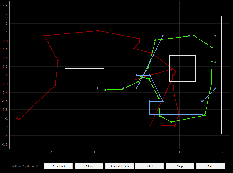
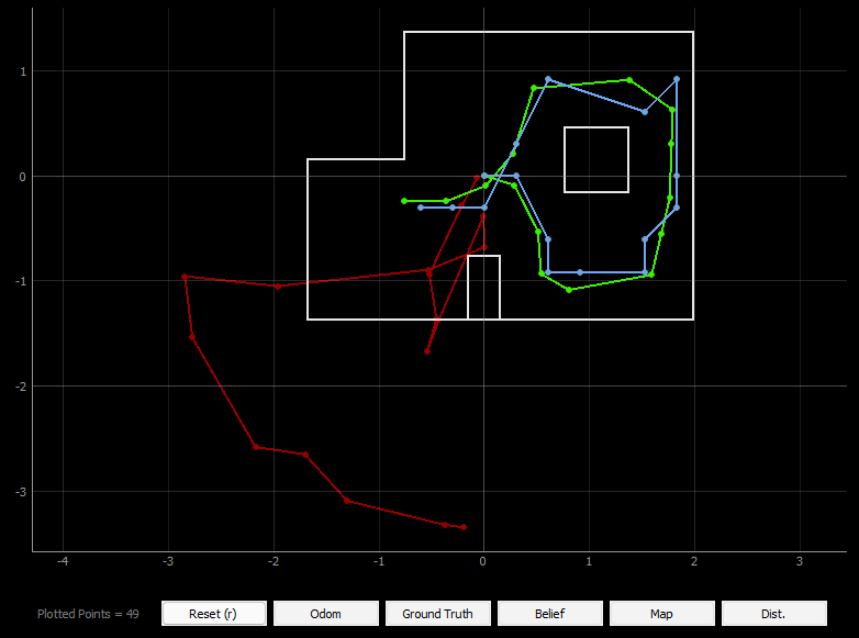
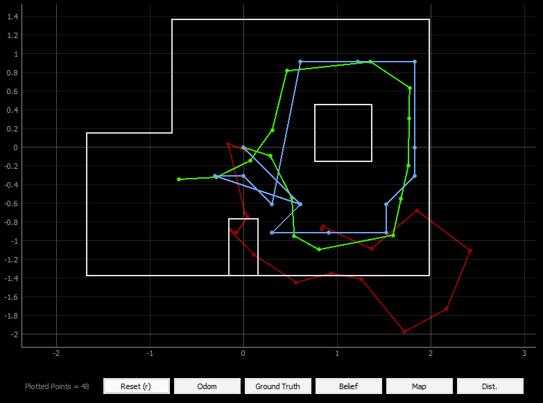
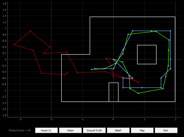
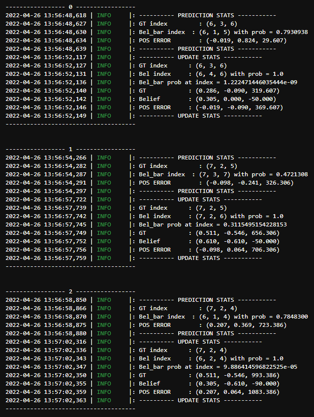
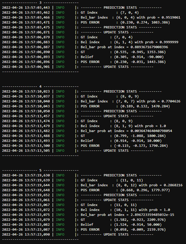
Even in the statistics for one of the trials we can see small amount of error and the robot's high confidence in its belief (almost always close to 1) which means that the localization is working well. A notable thing is that the POS ERROR for the angle was piling up to a large value. This is because the ground truth update in the angle is not normalized, and keeps getting increased after each run. After several trials, I found that the localization during a straight path in the trajectory is better than that in the corners, for example the top right and the bottom left corner in the trajectory. I wonder if the cause for this is ambiguity in the robots sensor measurement and the sensor model.

A useful feature to add to this codebase would be a way to visualize the bel and bel_bar probability distributions, similar to those shown in the lectures. For this lab, I was planning to add a 3D heatmap to do so, such that instead of only the highest belief index, we can see the robots belief across all the cells. This would help us monitor the change in robot belief, and also potentially determine the reason behind some of the discrepancies. While I was short on time to do this for lab 11, I plan to implement it in lab 12 for debugging purposes.

Overall, this was a more challenging lab than the previous few in terms of coding, however, not having to run and debug code on the robot was refreshing. I look forward to get back to it in the next lab as we implement the Bayes filter on the robot and try to localize.