LAB 12
Localization (Real)
Lab 12 was an exciting lab, where we implemented Bayes filter-based localization on the actual robot. Just like in Lab 11, where the simulator robot performed a trajectory and localized at every step, this lab was the first step of doing that on the robot in which we only executed the update step in the Bayes filter at different poses in the lab and observed the robot’s perception of its location. This was an interesting lab, where we saw for the first time the robot performing an autonomous task without much tuning or control required (like in PID).
In this lab, I worked with Aryaa Pai (avp34) and Aparajito Saha (as2537). We used my robot and the Artemis codebase from previous labs, and Aryaa’s and Apu’s Jupyter notebooks to control the robot and perform the localization on the system.
Localization Module
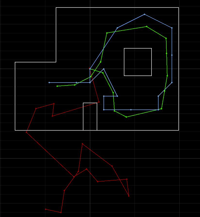
For this lab, the course staff has provided us with a fully functional and optimized Bayes filter implementation in the form of a Localization class along with wrapper classes VirtualRobot and RealRobot for handling the robot with the localization module. We have also been given a complete Jupyter notebook lab12_sim.ipynb that performs a trajectory with the virtual notebook and localizes at each step, similar to Lab 11. The result of one such run is shown below, where the green line shows the actual movement of the robot (ground truth), the red line represents the robot’s perception based on its odometry model, and the blue line represents the robot’s perception based on Bayes filter localization. The result is very similar to that in Lab 11, where the robot’s belief closely matches the actual movement in most portions of the trajectory.
Localization on the Real Robot
In order to perform localization on the real robot, we needed to complete the provided lab12_real.ipynb Jupyter notebook with the implementation of the RealRobot class. This class is used to interface with our robot through Bluetooth commands and prepares the data to be used for the update step in the Bayes filter, that is, the sensor model measurements taken around the current pose of the robot.
The implementation of the perform_observation_loop() function is shown below, which is called by the localization class in the update step for the robot to rotate on it’s spot and obtain 18 distance sensor measurements in the range 0° to 360°. In our implementation, this function sends the robot a command CMD.TURN_RECORD 18 times, which causes the robot to take a distance measurement, and turn by a preconfigured angle of 20° each times. Once the loop has been performed and the data collected, the function obtains all the measurement values to Jupyter using the CMD.GET_DATA command like in previous labs. We also added some helper functions to the class for the callback function and for PID tuning. The video below shows the robot performing one observation loop.
The obtained sensor values array needs to be modified to match the format used in localization, which is sensor readings at 20° increments like 0°, 20°, 40° counter-clockwise. Since Lab 6, the turning PID controller in my robot has been implemented such that it turns the robot clockwise for a positive target angle (corresponding to the placement of the IMU on the robot). Therefore, instead of re-orienting and retuning the controller on the robot, we chose to turn the robot clockwise to perform the observation loop – resulting in sensor data at 0°, 340°, 320° … – which is transformed thereafter. The sensor data array is reversed, and the last element (at 0°) put in the beginning to result in the final sensor_ranges vector returned by the function.
def perform_observation_loop(self, rot_vel=120):
    """Perform the observation loop behavior on the real robot, where the robot does
    a 360 degree turn in place while collecting equidistant (in the angular space) sensor
    readings, with the first sensor reading taken at the robot's current heading.
    The number of sensor readings depends on "observations_count"(=18) defined in world.yaml.

    Keyword arguments:
        rot_vel -- (Optional) Angular Velocity for loop (degrees/second)
                    Do not remove this parameter from the function definition, even if you don't use it.
    Returns:
        sensor_ranges   -- A column numpy array of the range values (meters)
        sensor_bearings -- A column numpy array of the bearings at which the sensor readings were taken (degrees)
                            The bearing values are not used in the Localization module, so you may return a empty numpy array
    """
    # Send commands to execute loop and record data
    for i in range(18):
        ble.send_command(CMD.TURN_RECORD, "")

        time.sleep(1)

    # Send command to obtain data -- stored in self.artemis_data
    asyncio.run(self.get_data("0"))

    # Transform the sensor data array to match the format of localization
    self.artemis_data.reverse()
    self.artemis_data = [self.artemis_data[-1]] + self.artemis_data[:-1]
    sensor_ranges = np.array(self.artemis_data)[np.newaxis].T

    return sensor_ranges, np.empty_like(sensor_ranges)
Results
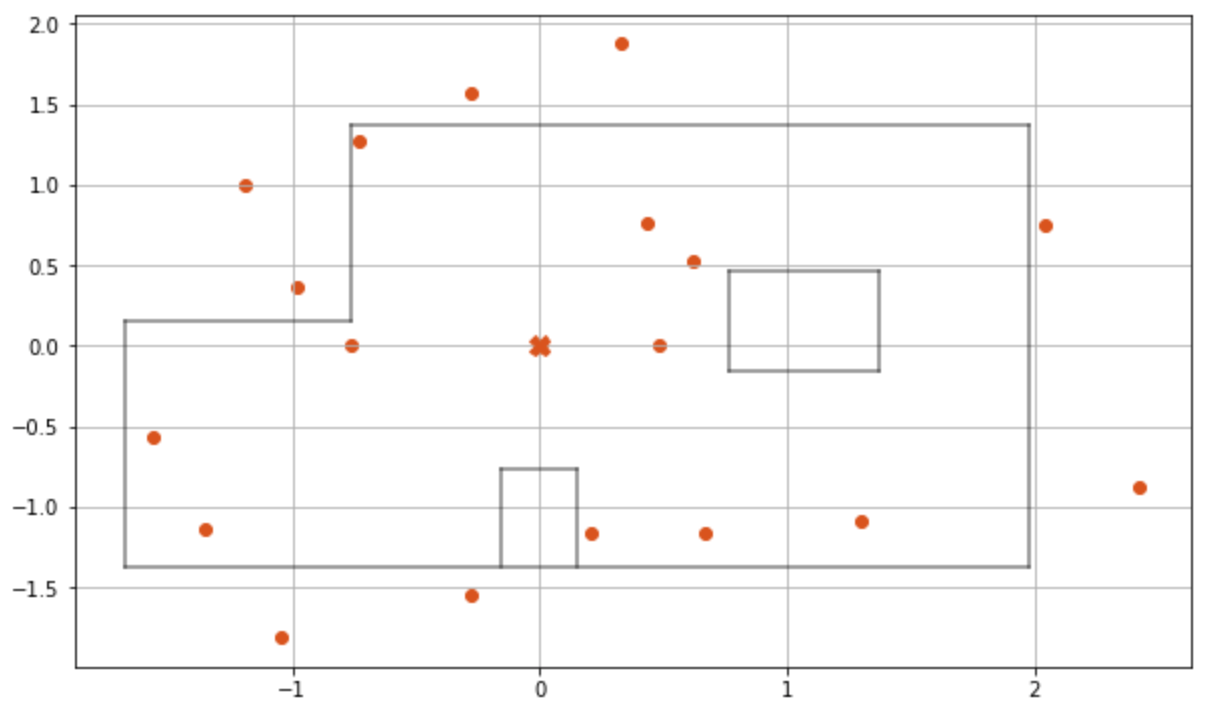
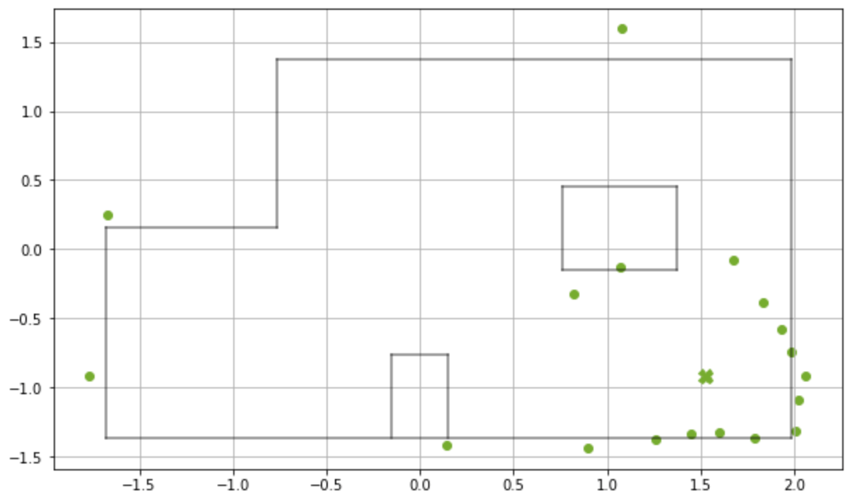
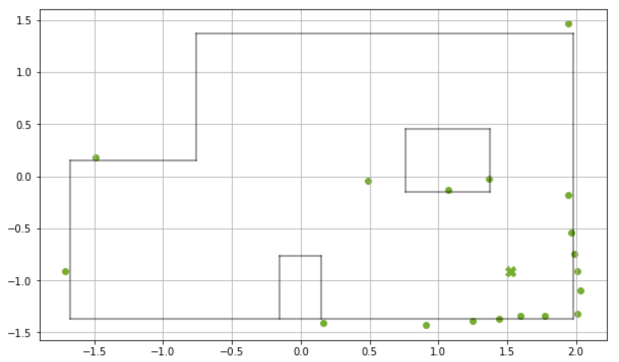
Once we had implemented and tested the RealRobot class, we could perform Bayes filter localization at the five designated markers (including the origin) in the lab and observe the robot’s perceived pose. In the update step, the localization module compares the obtained sensor ranges with all possible sensor ranges at every grid cell (x, y, θ) to estimate the current pose of the robot, or the belief. The table below shows the plot of the observation loop measurements and the results of the update step at each of the markers.
Marker
Observation Data
Update Step
(0 ft, 0 ft, 0°)
Update time :0.003 s
Bel index   :(5, 4, 8)
Prob        :0.9999999
Belief      :(0.0m, 0.0m , -10.0)
                or (0 ft, 0 ft, -10°)
(0 ft, 3 ft, 0°)
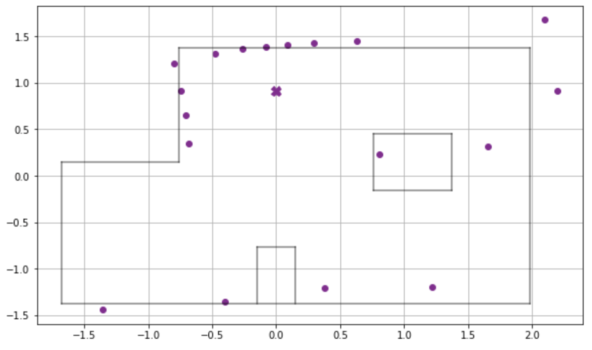
Update time :0.003 s
Bel index   :(5, 7, 8)
Prob        :1.0
Belief      :(0.0m, 0.914m , -10.0)
                or (0ft, 3ft, -10°)
(5 ft, 3 ft, 0°)
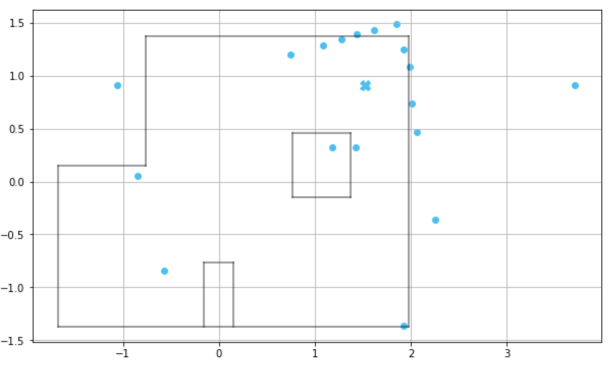
Update time :0.003 s
Bel index   :(10, 7, 8)
Prob        :0.9999994
Belief      :(1.524m, 0.914m , -10.0)
                or (5ft, 3ft, -10°)
(5 ft, -3 ft, 0°)
Update time :0.002 s
Bel index   :(10, 1, 8)
Prob        :0.9999999
Belief      :(1.524m, -0.914m , -10.0)
                or (5ft, -3ft, -10°)
(-3 ft, -2 ft, 0°)
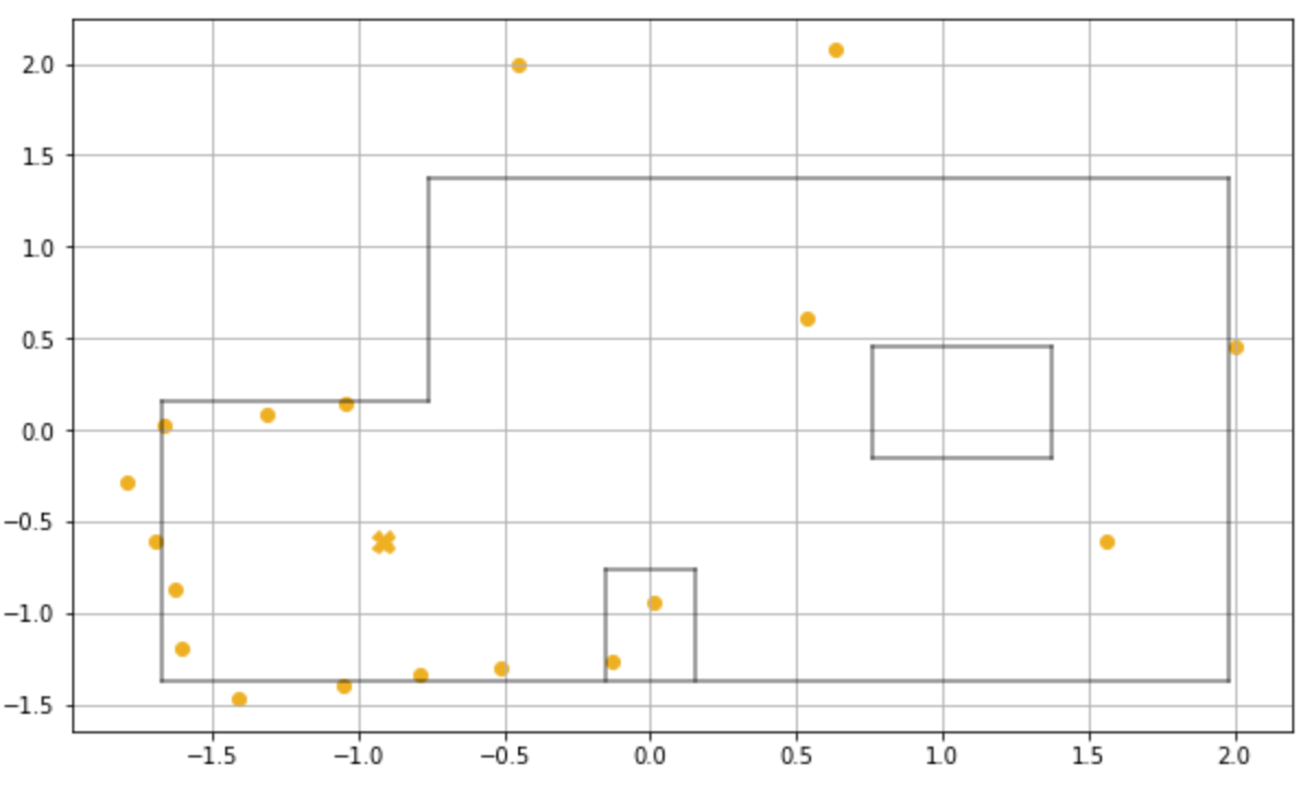
Update time :0.003 s
Bel index   :(2, 2, 8)
Prob        :0.9999999
Belief      :(-0.914m, -0.610m, -10.0)
                or (-3ft, -2ft, -10°)
(5 ft, -3 ft, 0°) Incorrect
Update time :0.002 s
Bel index :(8, 0, 6)
Prob :0.8859641
Belief :(0.914m, -1.219m , -50.0)
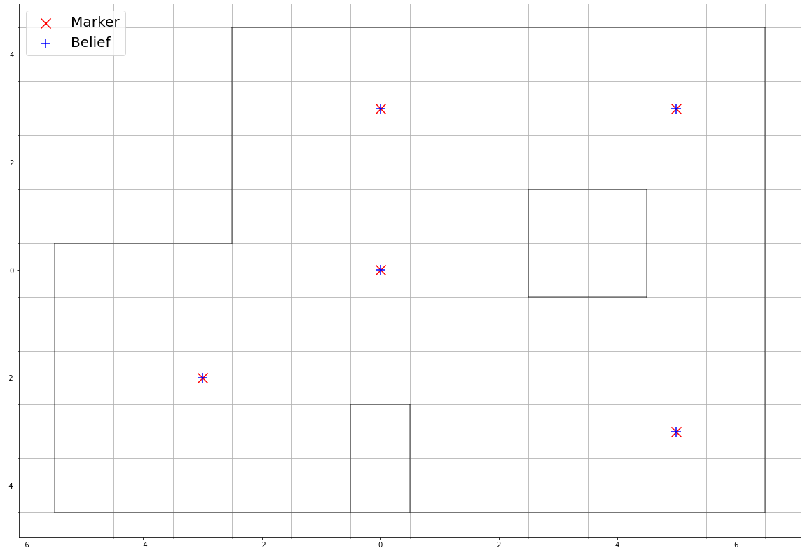
or (3ft, -4ft, -50°)As we can see in the table and the cumulative plot below, the robot is able to correctly localize at all five of the markers, even when the observation data doesn't perfectly match the boundaries of the room, that too with a very high certainty (probability almost 1.0). Frankly, this accuracy of this system took us by surprise as well, and we performed the localization multiple times on some of the markers to achieve the same result almost always. Seems like the Bayes filter update step and the sensor model of our robot work much better than we expected. The only error we saw were while localizing at (5 ft, 3 ft, 0°) as shown by the last entry in the table. After localizing a few times at this marker, we observed that the robot predicts correctly and incorrectly fairly equal number of times. The reason why the robot's incorrect belief at these locations is such is inexplicable, except for the fact that this is a marker neighboring a corner and the robot could potentially mistake itself to be in any one of the corners in the room. We plan to further test around this marker in the next lab and come up with a strategy to avoid significant errors in mapping due to this.
Another notable observation is that while the robot correctly localizes in the X and Y dimensions for all the markers, the angle belief is always -10° instead of the expected 0°. This is because of how the localization module and the grid model is structured in the lab. After talking with Vivek about this, we know that the angle space of 0° to 360° is divided into 18 subranges of the form 0° - 20°, 20° - 40°, and so on; however, these subranges are discretized with the value of their center angle resulting in the angle range being -30°, -10°, 10°, 30° etc. So, if the robot is at 0° angular pose, the result of the localization can only be either -10° or 10° because 0° doesn't exist in the angle space. For the next lab involving mapping along with localization, we may modify this to output the correct angle so that the robot movement doesn't cause drift inaccuracies.
This was an exciting lab and I'm (astonishingly) happy with the results of the localization. I'm looking forward to further upgrading this model to move the robot through a given trajectory using mapping and localization.