LAB 3
TOF and IMU
In this lab, we set up and tested the Artemis with two types of sensors that we will be using on the robot: two Time-of-Flight distance sensors and an Inertial Measurement Unit. The first part of the lab involved connecting these sensors to the appropriate pins of the Artemis. Both types of sensors communicate over the I2C protocol and could be connected in a daisy-chain fashion to the Qwiic connector on the Artemis board. We also had to consider the placement of all these components inside the robot to render their order in the daisy chain, and decide the length of wires required. My final hardware circuit is shown below.
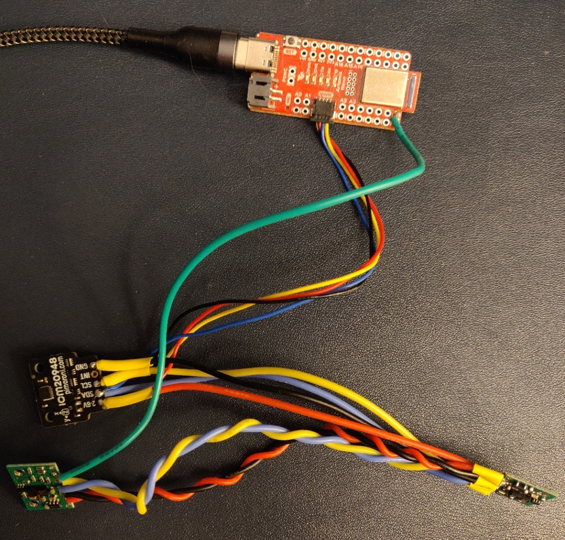
XSHUT pin of TOF 2 (green) wires back to a digital pin on the Artemis.ToF Setup
The Time-of-flight sensors VL53L1X are accompanied by a SparkFun library which can be downloaded from the Library Manager. Since there are two sensors connected to the Artemis and have the same I2C address, I turned off sensor 2 using an active-low signal on its XSHUT pin while testing sensor 1.
The TOF sensor has 3 modes of operation with different maximum ranges and their respective timing budget: short, medium, long. The short mode measures up to 1.3m and can support a timing budget of 20 ms, while the long mode up to 4m requires at least 140 ms for measurement (Figure 6 in VL53L1X datasheet). For our application, we need the sensor response to be as fast as possible (20 ms), and don’t necessarily need a very long range of 4m. Therefore, the short-range mode will work well.
Single ToF
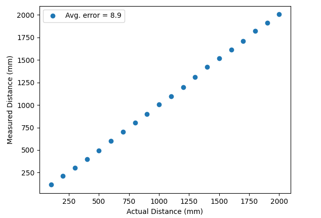
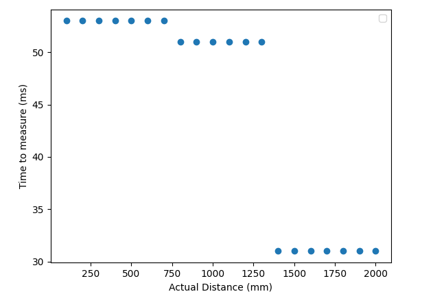
I used the Example1_ReadDistance and Example2_SetDistanceMode to test the ToF sensor with Artemis. The following code and plots show the accuracy, and ranging time of the sensor in the short mode.
In order to make the sensor sample faster and at a fixed rate, we can also set its timing budget using the setTimingBudgetInMs() function. If we set the the timing budget to its least possible value of 20 ms, the accuracy of the sensor remains fairly similar but all measurement occurs within 20 ms.
Two ToF Sensors
Since the two ToF sensors we use on the robot are the same, they come with the same default I2C address. A way to use both of them simultaneously is to change the address of one of the sensors, which can be done by shutting the other sensor off like earlier. This setup and its results are shown below.
// Artemis setup to communicate with two VL53L1X sensors simultaneously
#define DEF_ADDRESS 82  // Default address
#define NEW_ADDRESS 32

// Shut down sensor 2 first to change address of sensor 1
distanceSensor2.sensorOff();

// Change address if not already changed
int sensor1_address = distanceSensor1.getI2CAddress();
if (sensor1_address == DEF_ADDRESS)
{
  distanceSensor1.setI2CAddress(NEW_ADDRESS);
  Serial.print("Sensor 1 address changed to 0x");
  Serial.println(distanceSensor1.getI2CAddress(), HEX);
}

if (distanceSensor1.begin() != 0)
{
  Serial.println("Sensor 1 failed to begin.");
  while(1);
}
Serial.print("Sensor 1 online at 0x");
Serial.println(distanceSensor1.getI2CAddress(), HEX);

// Turn on sensor 2
distanceSensor2.sensorOn();

if (distanceSensor2.begin() != 0)
{
  Serial.println("Sensor 2 failed to begin.");
  while(1);
}
Serial.print("Sensor 2 online at 0x");
Serial.println(distanceSensor2.getI2CAddress(), HEX);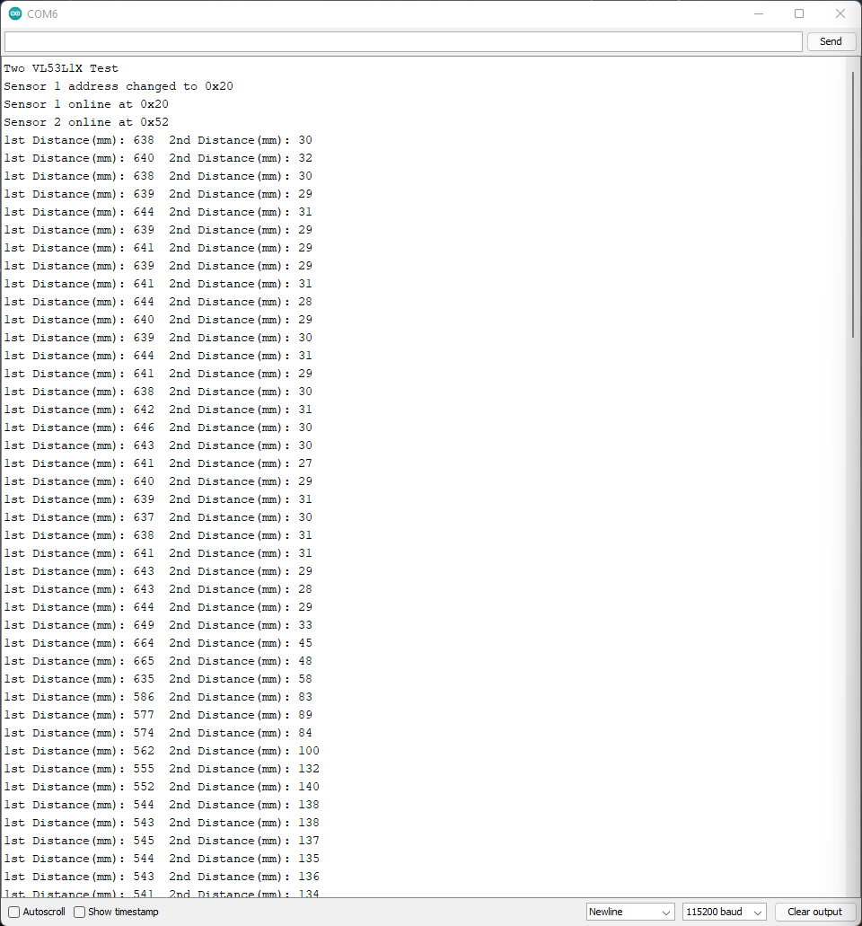
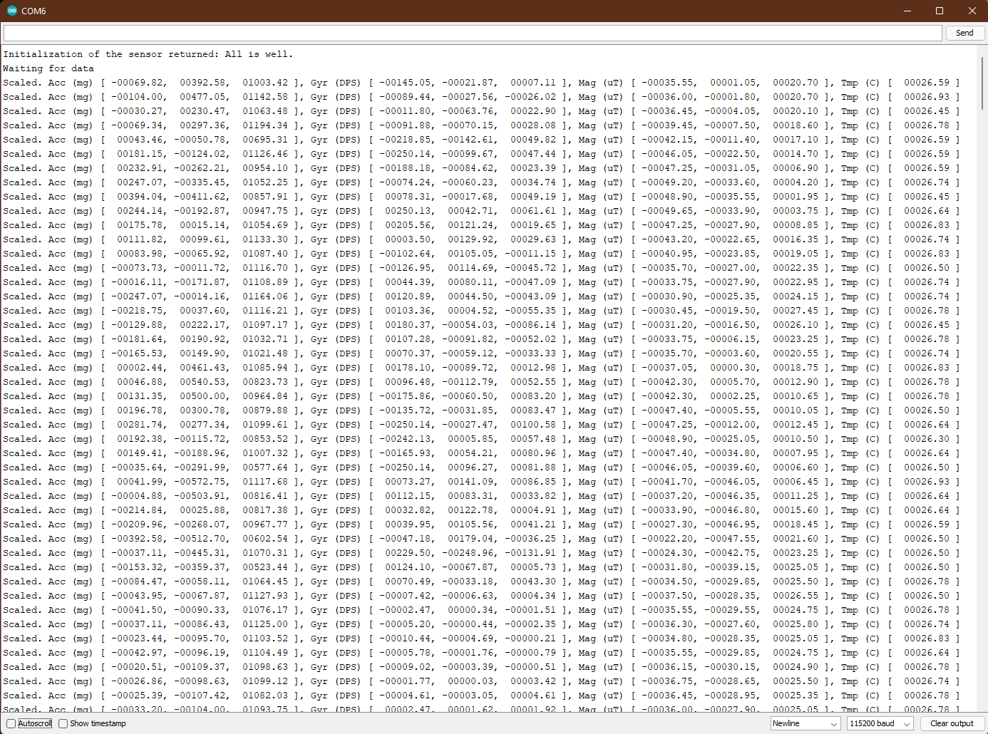
IMU Setup
The setup for the ICM20948 IMU sensor involved downloading the SparkFun library for it from the Library Manager on Arduino. I used the Example1_Basics.ino code that came with the library to test the sensor. This sketch simply prints out the measured values of accelerometer(3-axis), gyroscope (3-axis) and magnetometer (3-axis). To use this example with our breakout board, we need to set the value of AD0_VAL to 0 as the ADR jumper is closed.
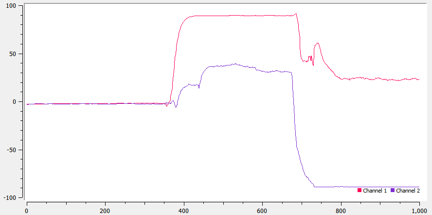
In the figure below, we can see how the sensor data changed as the sensor was rotated, flipped and moved around. The acceleration in the downward direction is high due to gravitational forces, therefore, whenever the sensor is laid flat on a surface, the z-axis acceleration is almost 1000 mg. The gyroscope values increase whenever we rotate the sensor along any of the axes.
Accelerometer
One of the three sensor on the IMU is a 3-axis accelerometer. With reference to the lectures, these values can be used to determine the pitch and roll of the sensor, as shown in the code snippet below.
// Pitch and roll calculation from accelerometer measurements
float pitch = atan2(sensor.accX(), sensor.accZ()) * 180 / PI;
float roll  = atan2(sensor.accY(), sensor.accZ()) * 180 / PI;
The pitch and roll measurements were not very accurate and had up to a 5° error when the sensor is held up right such that the pitch/roll are +90°/-90°.In order to correct this error, I used a two-point calibration method as suggested in the lab write-up, using the explanation on Adafruit. The implementation of this calibration and its results are shown below.
// Two point calibration on pitch and roll

// Values for sensor calibration
#define PITCH_RAW_HIGH 84.0
#define PITCH_RAW_LOW -85.0
#define PITCH_REF_HIGH 90.0
#define PITCH_REF_LOW -90.0

#define ROLL_RAW_HIGH 84.0
#define ROLL_RAW_LOW -84.0
#define ROLL_REF_HIGH 90.0
#define ROLL_REF_LOW -90.0

float pitch_corrected = ((pitch - PITCH_RAW_LOW) * (PITCH_REF_HIGH - PITCH_REF_LOW) /
    (PITCH_RAW_HIGH - PITCH_RAW_LOW)) + PITCH_REF_LOW;
float roll_corrected = ((roll - ROLL_RAW_LOW) * (ROLL_REF_HIGH - ROLL_REF_LOW) /
    (ROLL_RAW_HIGH - ROLL_RAW_LOW)) + ROLL_REF_LOW;
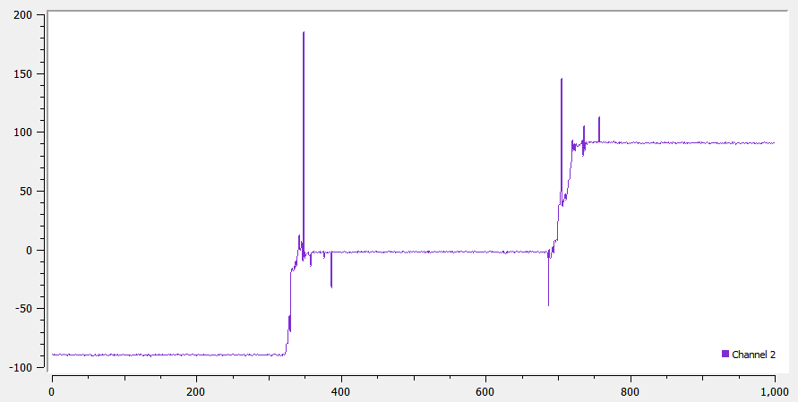
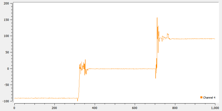
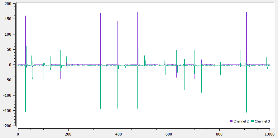
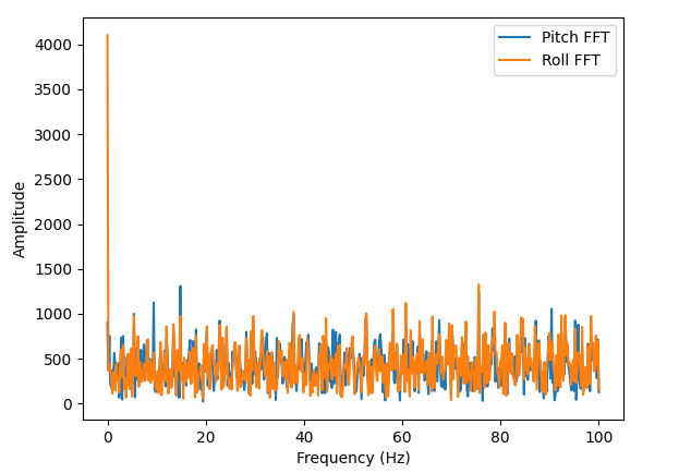
To correct for noise, we can analyze the frequency response of the sensor to find the noise frequency and filter it out. I did this by running the measurement loop continuously, and recording the values for time in milliseconds, pitch, and roll, and using that to calculate the FFT of the data. I found that although running continuously, the time interval between two readings was almost uniformly 5ms, thus resulting in a sampling rate of 200 Hz. The pitch and roll measurements with aperiodic taps, and the FFT of their measurements is shown below. As we can see, there is no distinct noise frequency in the spectrum. This is expected, as the sampling frequency of 250Hz is very low to record any high frequency noise.
To remove noise, we can use a low-pass filter over our measurements. Since it was not possible to determine the cutoff frequency of noise from the frequency response, I tried a few different values for α {0.5, 0.1, 0.05, 0.01} and observed how they responded. Higher the α, lower the magnitude of noise, while higher the response time to recover from the noise. Given this, the appropriate value seems to be 0.1, where the noise magnitude is reduced from being greater than 150, to below 50, and the system also recovers within a few ms.
// Implementation of low-pass filter on pitch and roll readings
float alpha = 0.1;

pitch_corrected = alpha * pitch_corrected + (1.0 - alpha) * pitch_old;
pitch_old = pitch_corrected;

roll_corrected = alpha * roll_corrected + (1.0 - alpha) * roll_old;
roll_old = roll_corrected;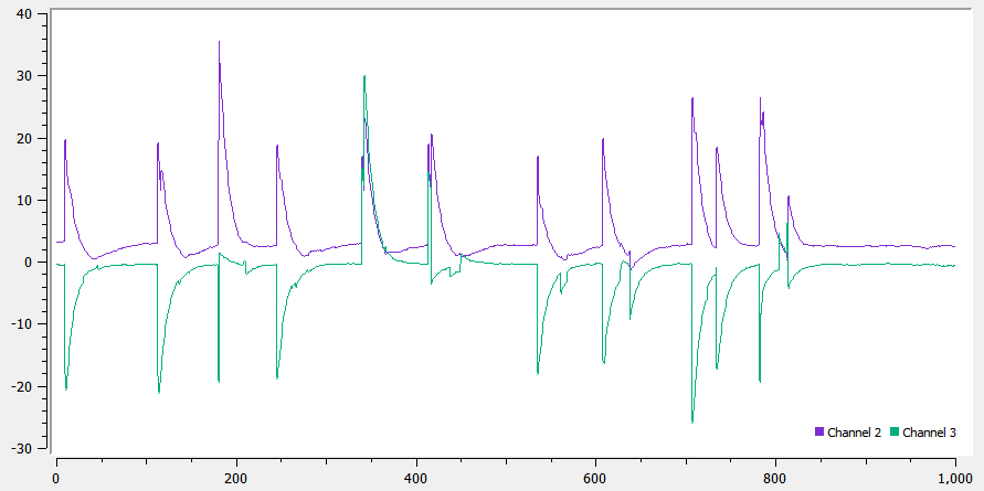
Gyroscope
The gyroscope measures the angular velocity along the 3-axes so used integration to calculate these angles form the equations discussed in class. From the plot of these measurements shown below, we can see that even when the sensor is kept stationary, the calculated angle values keep changing almost linearly. This is because the measured angular velocity is never exactly zero, and the integral keeps accumulating. As we increase the sampling rate, we see that the sensor becomes more susceptible to sudden changes in the angle.
// Using gyroscope measurements to calculate pitch, roll, yaw inside the main loop
int dt = millis() - last_time;
sensor.getAGMT();

roll  = roll - sensor.gyrX() * dt * 0.001;

pitch = pitch - sensor.gyrY() * dt * 0.001;

yaw   = yaw - sensor.gyrZ() * dt * 0.001;

last_time = millis();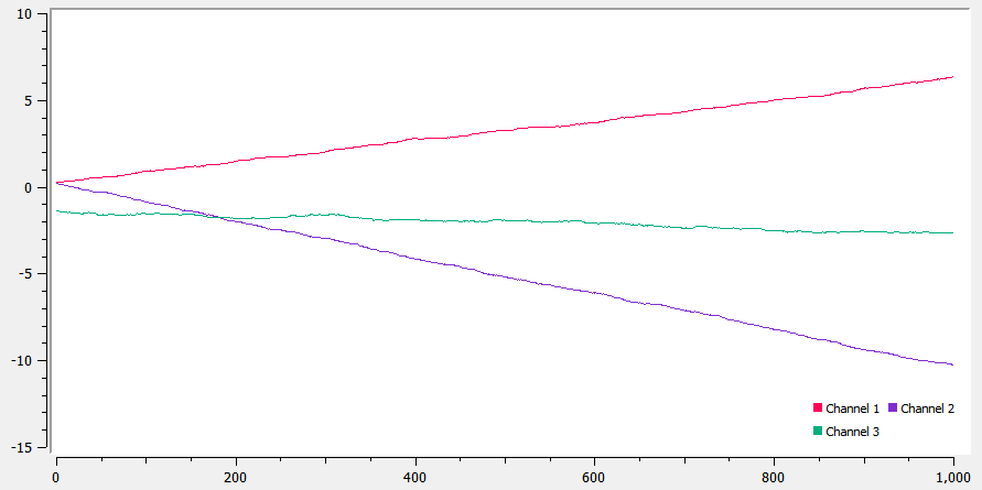
In order to fix this issue or drift, we can use a complementary filter that incorporates the pitch and roll angles calculated from the accelerometer as shown in the code snippet. Now, we can see that the measured angle remains almost constant and only spikes when the sensor orientation is changed.
// Using gyroscope and accelerometer measurements in a complementary filter to obtain pitch and roll

float alpha = 0.9;
float beta  = 0.1;


roll_gyr = roll - sensor.gyrX() * dt * 0.001;
roll_acc = atan2(sensor.accY(), sensor.accZ()) * 180 / PI;
roll_acc = ((roll_acc - ROLL_RAW_LOW) * (ROLL_REF_HIGH - ROLL_REF_LOW) /
    (ROLL_RAW_HIGH - ROLL_RAW_LOW)) + ROLL_REF_LOW;
roll     = (1 - alpha) * roll_gyr + alpha * roll_acc;

roll = beta * roll + (1.0 - beta) * roll_old;
roll_old = roll;

pitch_gyr = pitch - sensor.gyrY() * dt * 0.001;
pitch_acc = atan2(sensor.accX(), sensor.accZ()) * 180 / PI;
pitch_acc = ((pitch_acc - PITCH_RAW_LOW) * (PITCH_REF_HIGH - PITCH_REF_LOW) /
    (PITCH_RAW_HIGH - PITCH_RAW_LOW)) + PITCH_REF_LOW;
pitch     = (1 - alpha) * pitch_gyr + alpha * pitch_acc;

pitch = beta * pitch + (1.0 - beta) * pitch_old;
pitch_old = pitch;