LAB 7
Kalman Filter

Lab 7 was the second part of the 3-part labs 6-8, at the end of which we perform stunts with the robot. In this lab, we implemented the Kalman Filter, which can be used to make the robot controller faster with the help of probabilistic models based on inputs and observations. We first performed a step response on the robot, used the data from it to create a Kalman filter model on Jupyter notebooks, and then implemented the filter on the robot itself.

Step Response

The first part of the lab involved coding a step response in the robot, which meant running the robot forward at a constant speed (PWM). The robot had to move enough to achieve a constant speed and then stop a certain distance before a wall. Since I implemented Task B (Drift) in Lab 6, I didn’t already have a working PID controller for the robot to stop before a wall.

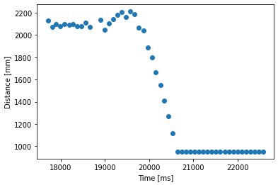
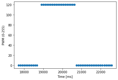
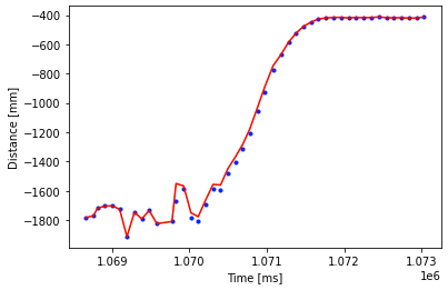
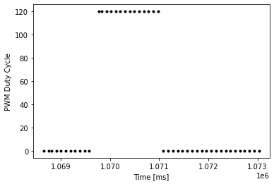
Starting from the code from Lab 6, I added another Bluetooth command for this behavior, called cmd.GO, both on the Artemis, and Jupyter. Once the robot receives this command, it first stays steady for 1 second, then starts moving forward until it is 100 cm away from the wall, and then it stops. Throughout this process, the Artemis records data about time, distance, and PWM speed, which can then be obtained on Jupyter through cmd.GET_DATA. I chose to run the robot at a constant PWM 120. Since this is a high speed and there is no PWM control, the robot actually overshoots significantly and stops very close to the wall, even with a large distance threshold of 100 cm.

// lab6.ino
// Segment of code from bluetooth command handler on Artemis 

From this step response, we can plot the distance measured by the TOF as the robot moves, and therefore the velocity, which can help us define the A and B state space matrices for the Kalman filter.

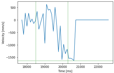
# Steady state speed = 1640 mm/s ==> d = 1 / 1640 
d = 0.0006

# 90% Rise time = 1.8 ==> m = -d * t_90 / ln(0.1)
m = 4.6903e-04 

A = np.array([  [0,1]   , 
                [0, -d/m]])
B = np.array([  [0] , 
                [1/m]])

Kalman Filter on Jupyter

Once we have the A and B matrices, we can implement the Kalman Filter on a Jupyter notebook, and test it on the data obtained from the step response. For this, I followed the discussion in the lecture and in the lecture slides to define a Kalman filter function that takes in the sensor reading, the PWM duty cycle, and the previous prediction, to output a new prediction in the model. The A and B matrices were discretized based on one instance of time difference dt. To start with, I used the process noise and sensor noise from the lecture, and as given in the lecture handout, I used matrix C for task B as shown below. After a few iterations, I was able to model the Kalman filter to fit the robot behavior pretty well. The final variables used and the result as follows.

C = np.array([[-1, 0]])

# Covariance matrices
sig_u = np.array([[50**2, 0], [0, 50**2]])
sig_z = np.array([[10**2]])

# Initial confidence
sig = np.array([[5**2, 0], [0, 5**2]])
# Initial state
x = np.array([[-dist_x[0]], [0]])

# Discretize A and B
Delta_t = dist_t[1] - dist_t[0]   # Sampling time
Ad = np.eye(2) + Delta_t * A
Bd = Delta_t * B

def kalman(x, sig, u, z):
    global Ad
    global Bd
    global C
    global I
    global sig_z
    global sig_u

    # Prediction step
    x_p   = np.dot(Ad, x) + np.dot(Bd, u)
    sig_p = np.dot(Ad, np.dot(sig, Ad.transpose())) + sig_u 

    # Update step
    KF = np.dot(sig_p, np.dot(C.transpose(), np.linalg.inv( np.dot(C, np.dot(sig_p, C.T)) + sig_z)))

    x_n   = x_p + np.dot(KF, (z - np.dot(C, x_p)))
    sig_n = np.dot((I - np.dot(KF, C)), sig_p)

    return x_n, sig_n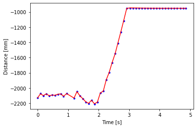

Kalman Filter on Artemis

After tuning the Kalman filter with noise and confidence parameters on the Jupyter notebook, I implemented it on the robot. For abstraction purposes, I created a class Kalman with all the state variables and parameters, as well as a function that can be called in the main loop to compute the next state. The BasicLinearAlgebra Arduino library mentioned in the lab handout was extremely useful to implement all the matrix calculations in the filter. Compared to the filter code in Jupyter, the main difference in the filter function when implemented on Artemis was that the discretization of the state space matrices was done in every instance. Since the duration of a TOF read can vary from a few tens of milliseconds to 130 milliseconds, using the correct time delta every time is expected to lead to more accurate predictions. However, this also add computation time to the filter function, and it might make more sense to use pre-discretized matrices in the future labs.

/** 
* Function to perform the Kalman filter 
*
* @param dt for discretizing
* @param u system output (PWM duty cycle)
* @param d current measured distance
* @return Derived value of predicted distance 
*/
float filter(int dt, int u, int d)  {
    Matrix<2, 2> Ad = I + A * dt;
    Matrix<2, 1> Bd = B * dt;

    Matrix<1, 1> u_ = {(float)u};
    Matrix<1, 1> z_ = {(float)d};

    // Prediction step 
    Matrix<2, 1> x_p = Ad*x + Bd*u_;
    Matrix<2, 2> sig_p = Ad*sig*~Ad + sig_u;

    // Update step 
    Matrix<1, 1> sig_m = C*sig_p*~C + sig_z;
    Matrix<1, 1> sig_m_inv = sig_m;
    Invert(sig_m_inv);
    Matrix<2, 1> KF_gain = sig_p*(~C*sig_m_inv);

    x = x_p + KF_gain*(z_ - (C*x_p));
    sig = (I - KF_gain*C) * sig_p;

    return x(0, 0);
}

When the step command GO was called, the Artemis repeatedly obtained data from the TOF and used it and the PWM at that time to compute the Kalman filter prediction. All of these values were logged and later retrieved to assess the filter as follows.

During the course of this lab, I faced numerous problems with my circuit on the robot, starting with connection issues on my I2C lines to the two TOFs, and later one of my motor drivers breaking down. I had to resolder the connections in my circuit a few times which delayed the process of tuning and testing the Kalman filter, and I had to finally do the entire process on a carpeted floor at my home. Before working on Lab 8, I plan to test and retune the filter by running the robot in Lab or the Phillips Hall corridors to get more appropriate parameters.