LAB 9
Mapping

Lab 9 is the first lab in the second half of the course with a focus on mapping and localization. In this lab, we use our robot to build a map of a room or arena set up in the lab space with information about the boundaries and the objects placed within. This was a very interesting lab and a new experience for me in robotics. It was super helpful that the course staff set everything up early and made sure that we utilize the time before spring break to get all the data points.

In the setup of the room, there are a few marked locations on which the robot needs to be placed and rotated, to get a series of distance measurements using the TOF sensor in the front of the robot. I chose to use my PID controller from Lab 6 to move the robot by fixed angle increments and take measurements. I worked on this lab with Aparajito Saha (as2537) and Aryaa Pai (avp34) for the data collection and manipulation.

PID Orientation Control

In Lab 6, I performed task B which involved turning the robot around by 180° using PID (I implemented PD). For this lab, I modified that code to do orientation control such that the robot turns over small angular increments, and takes a TOF distance measurement after each step. This was coded as a new Bluetooth command sent from the Jupyter notebook.

Ideally, the PID controller should turn the robot to reach the exact specified set angle. However, due to noise in IMU angular velocity measurement, I found that my controller had a constant linear offset in the angle, as I mentioned in Lab 6. Due to this, the robot turns 180° with a set point of 155° or 20° with a set point of 17°. After several runs with the same observation, I used this as a configuration and ran the control with the corrected set point. The robot turning from 0° to 360° over 20° increments can be seen in the video below.

As seen in the video, the robot doesn’t perfectly rotate on its axis, but instead the center of the robot drifts by a couple of centimeters from the marker, which may introduce error in the distance measurement. If the robot were placed in the middle of a 4x4m empty square, the displacement during the rotation will introduce up to 4-5 cm error for measurements on one side of the room (+180° from the starting orientation). We have also found the TOF to not be completely accurate, and it may further introduce an error of a few centimeters.

In order to deal with these potential errors, one solution could be to take more data points. Since the PID control on my robot was reliable for small angles, I turned the robot by 10° increments to get at least 36 data points from each marker, which worked better than 20° as discussed in the next section. One thing to note is that my PID controller turns the robot to its right, and therefore in the clockwise direction. Moreover, the starting angle for every mapping sweep was 180°, as seen in the video. Thus, the 36 angle increments were [170°, 160°, 150°, …, -160°, -170°, -180°].

Distance Measurement

Once the robot was able to spin properly over a set of increments, I added a distance measurement function after every turn. The robot was then kept to map distances from the 5 markers placed in the room at (0, 0), (-3, -2), (0, 3), (5, 3), (5, -3), and send the distance arrays to the Jupyter notebook over Bluetooth. The TOF sensor was placed in front of the robot and configured in the long-distance ranging mode like in the previous labs.

Since my gyroscope measurements were a little skewed, I didn’t use the measured yaw after every turn to associate with the distance measurement at that point to create the (R, ϴ) pairing. Instead, I equally divided up the 360° angle space into 36 angles at 10° increments and mapped the 36 distance values to the presumed angle space of [170°, 160°, 150°, …, -160°, -170°, -180°]. The small-angle increments and the greater number of measurements ensured that this hack didn’t introduce any significant error.

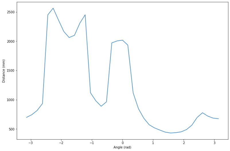
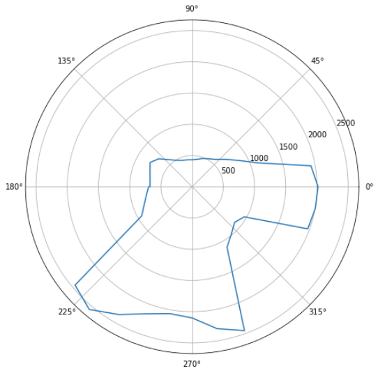
We first performed the mapping sweep with the robot from one marker point multiple times, to make sure that the movement and the distance measurement were reliable. Thereafter, we did the mapping from all 5 markers. The results from marker (0, 3) are shown below.

Creating the Map

After obtaining the distance mapping of the room from each of the markers, we needed to merge all the data to create a more complete map of the room. First, we had to convert the polar distance measurement from each marker to the inertial frame of reference in the cartesian form using transformation matrices. We were not too familiar with transformation matrices, so after talking with Vivek, we did a more manual conversion which worked just as well. The conversion algorithm, and its usage for converting and plotting the map from marker (5, 3) are shown below.

# Conversion of distance at different angles (polar) to cartesian coordinates in the inertial frame 

# Offset of TOF from center of the robot: DIST_TOF
# Location of marker: xo, yo 

for d, theta : (distance, angles):
    d = d + DIST_TOF 

    x = d * cos(theta) + xo 
    y = d * sin(theta) + yo 

    return x, y 

# Code to convert and plot the data collected from marker (5, 3)

# Convert marker position to mm
x0 = feet_to_mm(5.0)
y0 = feet_to_mm(3.0)

# Load the data 
distance_5_3 = np.array([...])
angles_5_3   = np.array([...])

# Convert to polar coordinates 
xs_5_3, ys_5_3 = polar_to_cartesian(angles_5_3, distance_5_3)

# Translate readings with the marker 
xs_5_3 = xs_5_3 + x0 
ys_5_3 = ys_5_3 + y0 

# Plot the data points 
plt.grid()
plt.scatter(xs_5_3, ys_5_3)

# Plotting the marker 
plt.scatter(x0, y0, marker='+')
    
plt.show()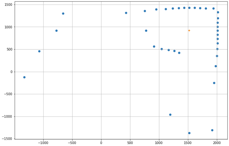 

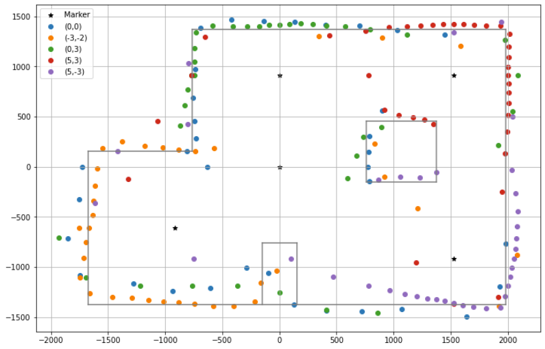
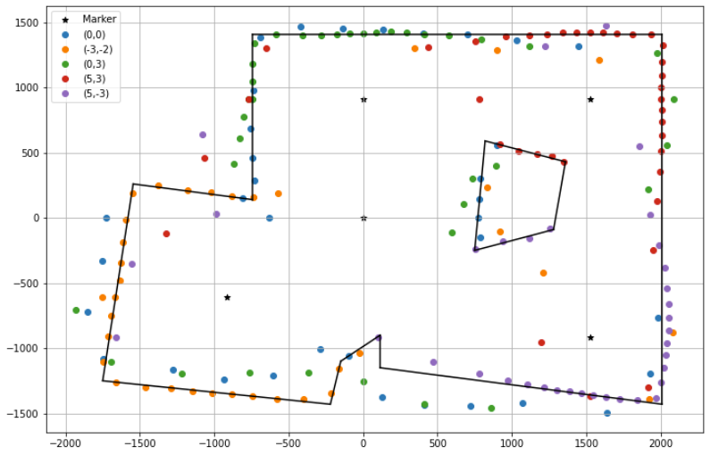
Once this plot was created for each of the markers, we plotted all of them on the same figure along with the actual room grid for reference. As we can see, the mapping procedure generated a somewhat acceptable result with a few inconsistencies. While the boundary of the room seems to be mostly appropriately mapped, there is not a very clear shape of the two boxes placed in the room.

From the mapping generated by the robot, we can create the robot’s own perception of the room as a line map. This will slightly vary from the actual map of the room because of the inaccuracies in the distance measurement. However, it will be more suitable to use this robot map in the simulator for future labs, as it better represents the perception of the robot. There can be multiple ways to find the lines of best fit to derive the map from the data points. I considered using linear regression to find the actual lines of best fit for different subsets of the points but abandoned the idea due to time constraints.

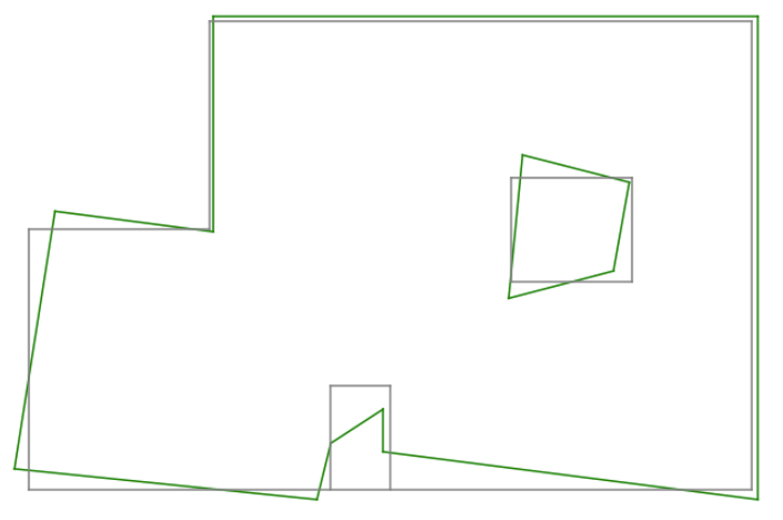
First, I tried determining all the lines in the map by direct observation of the point clusters, giving more priority to points measured from a nearby marker. For example, red points given more priority in the top right corner, while orange ones in the bottom left. This resulted in the map shown below, in which the top and right edges are straight like in the actual map, while all the other edges are distorted. This can be an acceptable map of the room.

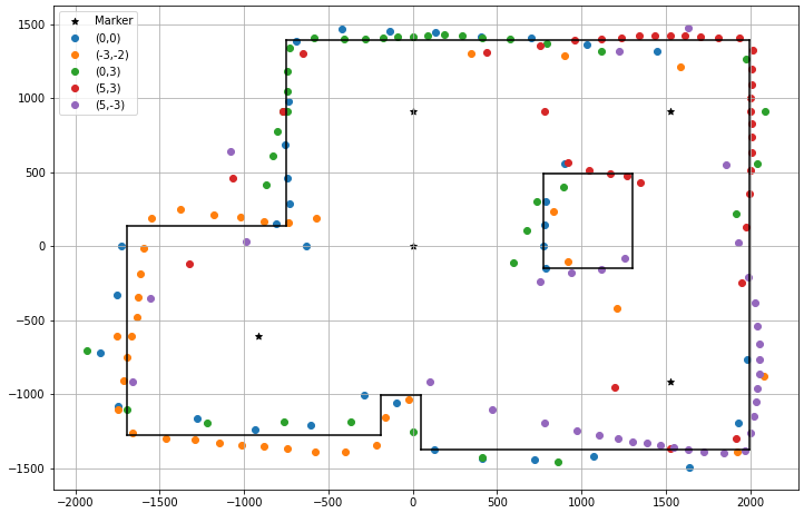
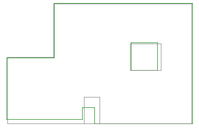
I also developed another type of mapping with the data, based on the prior knowledge that all the corners in the room are right angles, thus resulting in only vertical and horizontal edges. In order to do this, I selected a cluster of points that represent an edge, and averaged their x/y coordinate to obtain the constant parameter of the edge. For example, in order to compute the position of the right edge, I took all the data points on the right side and averaged their x-coordinate. Similarly, the y coordinate for all horizontal edges. This results in a map that matches very well to the true map of the room, especially at the boundaries of the room. This method also required careful selection of the points to be included in each cluster, while ignoring signicantly inaccurate, or misplaced measurements. Even so, due to the lack of data points around the middle box and the nook at the bottom of the room, the mapping of those areas is noticeably inaccurate.

This was a really fun lab! I hope that the line maps created of the room using the robot in this lab will work well for the tasks in future labs.